In 1911, the Serb Milutin Milankovitch sat down with friends and celebrated that a mutual friend had published his first collection of poems. Over a bottle of wine, he says “I can make a mathematical model, which can calculate the climate for all past and all future”. Perhaps he regretted it the next day, for this was the beginning of a 40-year effort to develop what is now called the Milankovitch theory. Milankovitch was a civil engineer, who calculated concrete structures, taught at the university, and took assignments for the defense in Serbia. Climate calculations became a hobby project, which eventually took over.

The discovery of ice ages

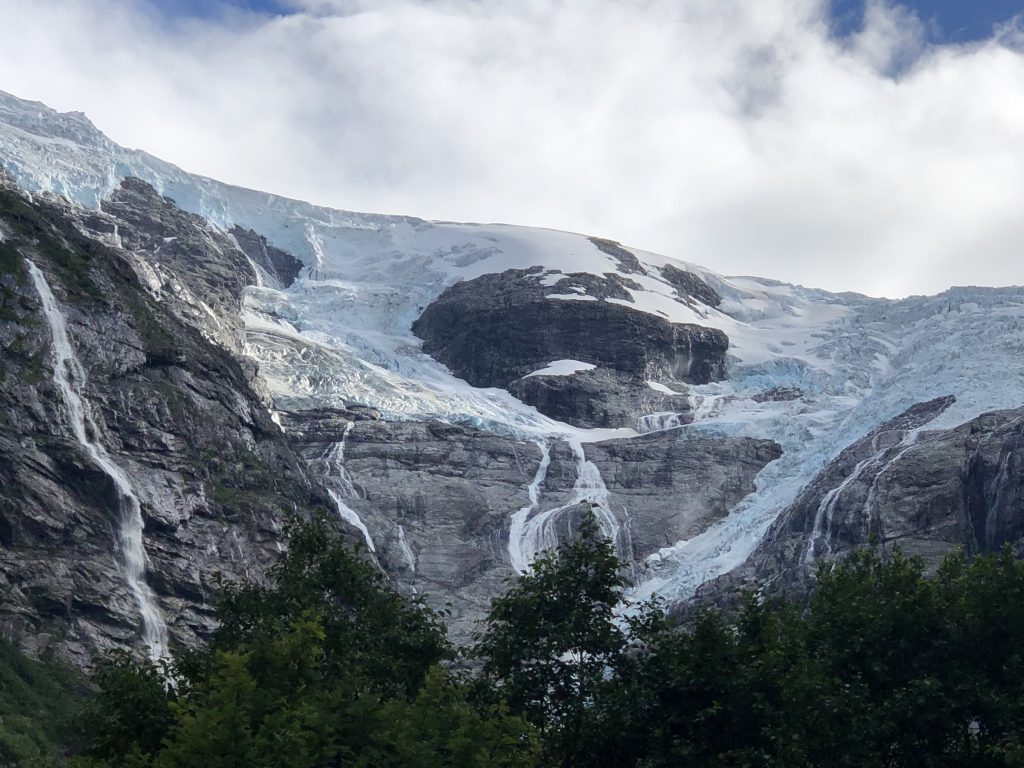
Figure 1. Melting glassier in Norway

In the middle of the 19th century, some geologists began to discuss what could be the origin of huge rocks that lay around Europe. It was a shock to the geologists, when they realized that these were remnants of the ice edge from a distant ice age. The ice edge around the North Pole had once stretched far down in Europe. The prevailing view was that the climate on Earth had an equilibrium state, with small variations over time. The discovery of a prehistoric ice age indicated that the climate had varied greatly. Today’s climate lasted for short periods, within long cold climate periods. During the last ice age, large parts of Scandinavia were covered by a 3,000-meter-thick ice sheet. New cold climate periods, and a new ice age, were thus a real possibility

Explanations of ice ages

In the 19th century, one began to discuss possible explanations. The question was whether the explanation could be changes in the radiation from the sun. The moon and the periods of the planets in the starry sky had been used as a calendar for several thousand years. Kepler had discovered that the earth moves in an elliptical orbit around the sun. Eventually one became aware that mutual gravity between the earth, the sun and the moon could change the shape of the earth’s orbit around the sun, and the inclination angle of the earth that regulated summer and winter. The problem was to perform necessary climate calculations. 

Research in prison

Milankovitch was born in Serbia and became involved in World War I. One day he was studying acts of war at the front. He must have had his own thoughts, because suddenly he imagined how he could make the calculations for the climate model. While visiting his hometown, he was arrested by the Austro-Hungarian army and imprisoned. In prison, he received a pen and paper, and began work on countless calculations to develop a climate model. After half a year in prison, and 4 years in house arrest, he was able to present his astronomical climate model. The model explaining ice ages was first published in 1920. The reception was not quite as he had expected. Periodic changes in the solar system, which cause ice ages on Earth, were beyond comprehension for most people.

Milankovitch theory

The short version of the Milankovitch theory is that the length of winter and summer varies over time. The angle of inclination of the Earth’s axis determines summer and winter in the north and south. In the north, it is summer when the earth’s axis points towards the sun on 23 June and winter when it points away from the sun on 21 December. The angle of inclination of the earth’s axis is now 23.4 degrees. It moves between 22.1 and 24.5 degrees over a period of approximately 41000 years. The angle had a maximum approximately at the year 8700 BC and gets a minimum approximately at the year 11800 AD. When the angle of inclination is reduced, we gradually get colder summers in the north. As a result, the winter distribution of ice in the north does not have time to melt in the summer, so that Arctic ice builds up gradually from year to year.

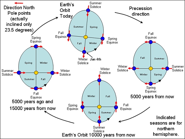
Figure 3: The Earth orbit rotation

The earth moves in an elliptical orbit around the sun. Highest speed, closest to the sun. Least speed, furthest from the sun. The elliptical orbit rotates with a period of about 20940 years. In the year 2022, the earth is closest to the sun on January 4, and furthest from the sun on July 6. When the Earth’s orbit has the highest speed during the winter months in the north, we get shorter winters, longer summers, and less growth of Arctic ice in the north. The direction of the Earth’s axis towards a fixed star rotates with a period of about 23,000 years. In the north, we now have midwinter on December 21, when the earth’s axis points most away from the sun. Around the year 12000 AD. the earth’s axis points maximally towards the sun and we get midsummer on December 21st. Midsummer closest to the sun, leads to a shorter summer period, and a colder climate in the north. The sum of the three cycles determines the time of ice ages, cold and warm climate periods in the north.

The Climate Clock

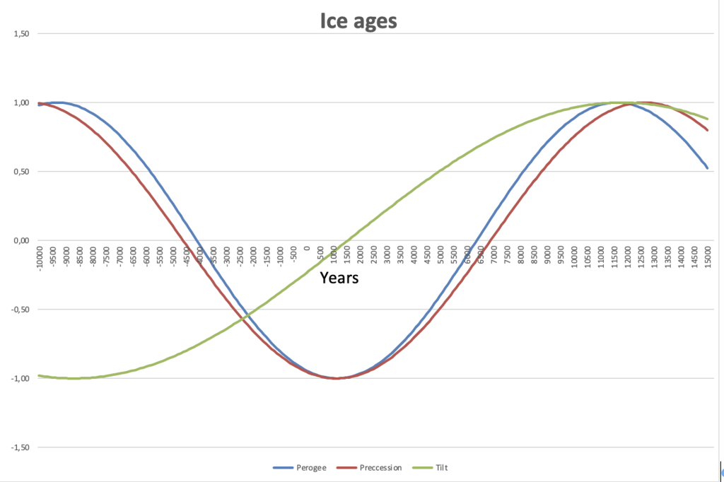
Figure 4. Ice ages and a warm period from 10000BC to 1500AD controlled by Perigee, Precession and Tilt.

The periodic changes are related to each other, much like several hands on a clock, where hands rotate at their own speed. When all hands point towards a warm climate, we will have a warm climate period. When all hands are aimed at a cold climate, we have ice age. I have created a simple climate model. It shows that the last ice age lasted from about 40,000 to about 18,000 years BC. The warm climate period came from about 4000 BC to about 1600 AD, with a maximum of about the year 500. The time 4000 BC coincides with the beginning of the first great civilizations, which were based on agriculture. The model says that the next ice age comes from about the year 6000 to about the year 20,000 AD, with a maximum cold period about the year 12,000. The next warm climate period is calculated for the years 22,000 to 27,000 AD.

The perfect ice age

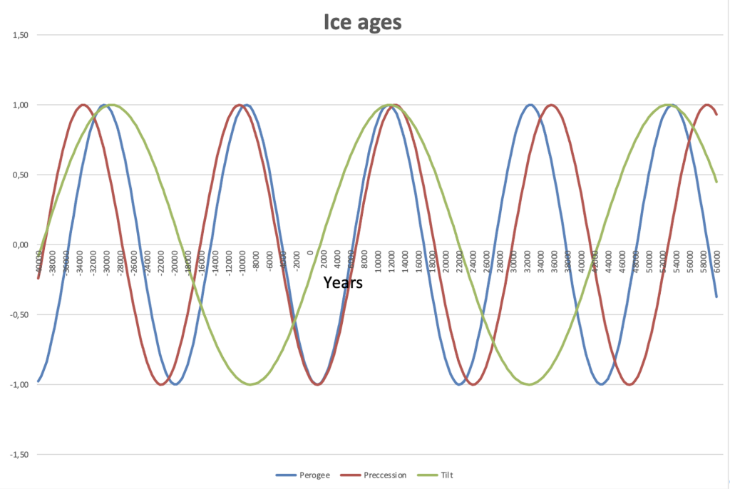
Figure 5. Five ice ages controlled by phase coincidences between Perigee, Precession and Tilt. The figure reveals that the upcoming ice age represents a “perfect” ice age when all periods have a maximum coincidence at the year 12000 AD.

Figure 5. Five ice ages controlled by phase coincidences between Perigee, Precession and Tilt. The periods have constructive interference close to the years 3600BC-26000BC, destructive interference close to year 10000BC and a “perfect” constructive interference at the year 12000AD. The time difference between the ice ages is close to 32000+12000=46000 years.

After Milankovitch

It would take 50 years before the Milankovitch theory was confirmed. In the 1970s, one began to analyze ice core samples from Greenland, which showed climate change over thousands of years. Here one found the periodic changes that confirmed the Milankovitch theory. The Milankovitch theory laid the foundation for modern climate science and a new understanding of the climate. The climate has no normal state, radiation from the sun varies over time and the climate is not controllable. After Milankovitch, astrophysicists, solar scientists, geographers and mathematicians were given more climate data series and better analysis methods. Today we see new climate machines where the planets affect radiation from the sun and the moon controls the temperature distribution in the ocean currents, in periods from hours, to several thousand years.

References

1. Gribben, John and Mary. 2001. How a change of climate made us human. Perguin Books. 
2. Hestmark, Geir. 2017. Istidens Oppdager. Jens Esmark, Pioneren i Norges Fjellverden. Kagge Forlag AS.