
The Earth´s global temperature has no mean value. Glaciers in the western part of Norway started to grow 500 B.C. The ice extent had a maximum temperature at the year 1755 A.D. [1], when the Greenland temperature had the coldest period in 4000 years. The cold period, known as “The Little Ice Age”, covers the period from approximately 1200 to 1850 A.D. The global modern warming temperature from 1850 to 2020 thus represents a temporary recovery period after “The Little Ice Age”.
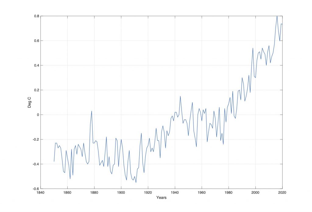
Figure 1. The Earth’s global mean temperature from 1850 to 2020.
The Earth’s global mean temperature (HadCRUT4) is estimated from the year 1850 to 2020 (Figure 1). The data series is based on sea temperature and land temperature records in a 5° by 5° global grid supported by the Climatic Research Unit [1]. The Earth’s global mean temperature (GMT) increased by approximately 1.0°C from 1850 to 2020. There was cold period from 1850 to 1920, an increased temperature from 1920 to 1940, a reduce temperature from 1945 to 1976, and a new increased temperature from 1976 to 2020 (Fig. 1).
The origin of the global temperature variations has been discussed for more the hundred years. Some fundamental research questions are:
- Is the global warming caused by human activities [2] or by natural variations?
- Is the global warming random or deterministic?
- Is the global warming controllable?
- What is expected upcoming temperature events the next decades?
The answers are hidden in the data series. All data series have a unique signature, which reveals the source of variations. If the source has deterministic variation, we can compute upcoming events.
Climate periods
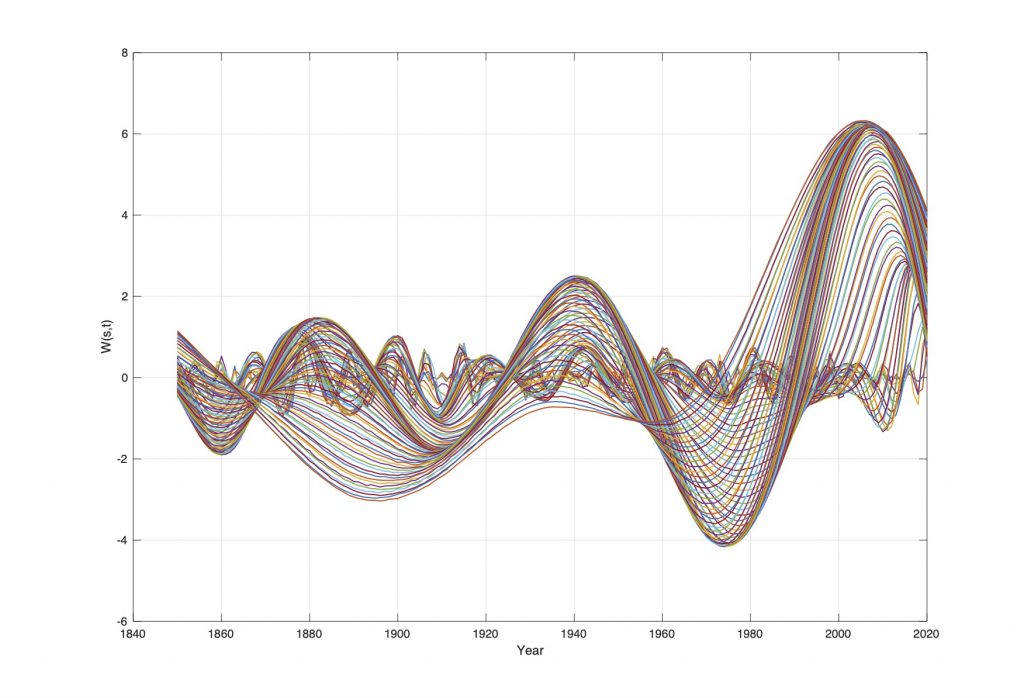
Figure 2. The computed wavelet spectrum of Earth’s global mean temperature from 1850 to 2020.
The data series signature is revealed in the data series period spectrum. Periods in the Earth´s temperature data series are separated by the wavelet transform:
where x(t) is the global temperature data series and Y() is a coif3 wavelet impulse function. The computed wavelets represent moving correlations between the data series x(t) and the scaled wavelet functions Y(), where the parameter a represents scaling period and b represents the scaling start position.
Dominant computed wavelets have phase shifts W(s(max, +0, min, -0), t) and WP(s(max, 0), t) as shown on Figure 2. Stationary periods in the wavelet spectrum W(s, t) are identified by computing the wavelet autocorrelations: WR(R(s), m) = E[W(s, t)W(s, t + m)], where WR(R(max), T) represents the maximum correlations R(max) to the dominant periods T in the wavelet spectrum W(s, t) (Figure 3).
The computed wavelet spectrum Wgt(s, t), shown on Figure 2 has minima and maxima close to: Wgmt(s(min/max), Fgmt()) = [(-2.0, 1860), (1.5, 1882), (-2.0, 1910), (2.5, 1940), (-4.0, 1974), (6.0, 2007)]. The wavelet spectrum reveals a stationary temperature variation of approximately 60 years. The source of the stationary period is revealed by computing the autocorrelations of the computed wavelet spectrum.
Climate signature
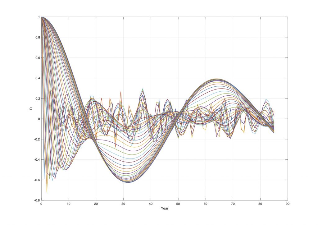
Figure 3. Computed autocorrelations Earth’s global mean temperature wavelet spectrum.
The autocorrelations WAgt(R(s), m) = E[Wgt(s, t)Wgt(s, t-m)] of the wavelet spectrum Wgt(s, t) computes the correlations R(s) in time distances of m years. The computed autocorrelations of the computed wavelet spectrum Wgt(s, t) has maximum correlations for: WAgmt(R(max), Tgmt) = [(0.22, 9), (0.23, 18), (0.16, 28), (0.30, 37), (0.20, 46), (0.12, 57), (0.38, 64), (0.16, 74)]. The global temperature variations to 1850 to 2020 have the correlations: R() = [0.22, 0.23, 0.16, 0.30, 0.20, 0.12, 0.38, 0.17] to the identified stationary periods: Tgmt() = [9, 18, 28, 37, 46, 57, 64, 74]. The identified stationary periods Tgmt() have coincidence to the period spectrum: Tgmt() = [1/2, 1, 2/2, 3/2, 4/2, 5/2, 6/2, 7/2, 8/2…]18.61 years. All global temperature variations from 1850 to 2020 are controlled by the number 18.61.
Climate Signature from the Moon
Mutual Earth-Moon-Sun (EMS) gravitation causes a spectrum of stationary tide periods in the Earth’s oceans. The period 18.61 is related to the 18.61-year nutation of the Earth’s axis (i.e., the Earth’s nutation causes a global 18.61-year tide between the poles and equator). Stationary long-period tides introduce vertical temperature mixing between warm surface temperatures and cold bottom temperatures, and thus, heat is redistributed throughout the large-scale oceanic thermohaline system. The lunar nodal tide signature in the global temperature spectrum reveals the lunar nodal tide as the source of global temperature variations.
The source of climate variations
The lunar signature spectrum in global temperature variability reveals that climate variations from 1850 to 2020 has a major influence from lunar forcing temperature variations.
Global warming control
The lunar signature in the global temperature variations is controlled by the Moon. Global temperature variations are not controllable, since the Moon is not controllable.
Deterministic climate variations
The lunar signature periods in the global temperature variation from 1850 is deterministic. The global temperature variations then have deterministic variations. The implication of deterministic variations are better forecast of upcoming temperature variations.
Upcoming climate variations
The dominant 64-year temperature period has maxima at the years: [1940+[Tgmt(64), 2Tgmt(64)…] = [1940, 2004, 2069…] (yr.) and minima at the years: 1974+[Tgmt(64), 2Tgmt(64)…] = [1974, 2038, 2102…] (yr.). Longer data series will explain interference from solar forcing temperature variations.
The NAO index from 1822 has the lunar forcing periods [1, 4, 6]18.6 (yr.)[4], North Atlantic Water [5],[6], Arctic ice edge position from 1579 has the lunar forcing periods [1, 4, 12]18.6 (yr.), Greenland temperature from 2000 B.C. has the lunar forcing periods [1, 4, 8, 12, 24]18.6 (yr.). This confirms lunar forcing climate variations up to 446 years or more.
Harald Yndestad
March 10, 2021
Literature
- Nesje, A., Bakke, J., Dahl, S O., Lir, Ø., & Matthiews, J A., (2008) Norwegian mountain glaciers in the past, present and future. Global and Planetary Change 60, 10-27.
- Climatic Research Unit (http://www.metoffice.gov.uk/hadobs/hadcrut4/).
- Scientific consensus on climate change. Wicipedia. https://en.wikipedia.org/wiki/Scientific_consensus_on_climate_change
- Yndestad, H. (2006). The influence of the lunar nodal cycle on Arctic climate. ICES Journal of Marine Science, 63(3), 401–420. http://doi.org/10.1016/j.icesjms.2005.07.015
- Yndestad, H., Turrell, W. R., & Ozhigin, V. (2008). Lunar nodal tide effects on variability of sea level, temperature, and salinity in the Faroe-Shetland Channel and the Barents Sea. Deep-Sea Research Part I: Oceanographic Research Papers, 55(10), 1201–1217. http://doi.org/10.1016/j.dsr.2008.06.003
- The Climateclock.no/Library
These combined with cloud coverage and Svensmark study prove that CO2 attribute is minute if any at all. But it would be interesting to see model estimate for the next wave, will it increase in amplitude as the last one is bigger than previous ? or will we see a decrease ?
The amplitude is controlled by solar variations, which explains the increased amplitude at 2020.
Next max is expected to be a colder period.