The Paris agreement is an international agreement to control global warming by reducing emission of CO₂ into the atmosphere. The aim is to limit global warming to 1.5-2°C, compared to “preindustrial time”. Before 2050 there must be a “balance” between emissions and absorption of CO₂ in the atmosphere. 

Accumulation of global temperature and accumulation of atmospheric CO₂ are dynamic systems. Control of dynamic systems are dynamic control problems. To control a dynamic system, the system must observable, controllable, and have minor disturbances from unknown sources.

Newton dynamics

Newton dynamics is widely used in physics, electronics, economics, logistics, and control in cybernetic systems. Climate science has not succeeded to develop reliable climate models. To understand why climate models are special, we must understand the Newton dynamic paradigm.

Ballistic movement

Isaac Newton (1642-1727) is described as the first modern scientist. He was born in Lincolnshire and for most of his life he studied ancient religion doctrines, the chronology of ancient kingdoms and ancient scientific works. He believed that an old divine knowledge was lost and some of it had been filtered down to Pythagoras, whose “music of the spheres” he regarded as a metaphor for the law of gravity. 

In Principia Mathematica Isaac Newton identified gravity as the First Cause, the indivisible force, without parts and without magnitude. The force that has the power to transform the universe. Newton discovered that inertial energy is stored in the movement of masses. To prove this theory, Newton invented differential equations to describe dynamic motion in nature. If the first movement is known, a chain of next movements may be computed. A deterministic chain of movements, described by mathematics.

Newtonian dynamics can be represented by a simple differential equation: dx(t)/dt = a*x(t)+u(t), where, a, represents the inertia of the velocity and u(t) represents the forced velocity from an external source. The speed can be calculated by a simple numerical integration, (x(t + T)-x(t))/T = a*x(t) + u(t), where T is the sampling period T = [t1- t0].

Newtons second law F=m*g computes how a force, F, and a mass, m, introduces a movement change: g = dx(t)/dt. The first movement is controlled by gravity, the invisible force without parts and magnitude. The final cause is controlled by the gravity direction. The movement speed, x(t), is preserved when the force, F= 0. The mass, m, represents  the movement “memory”. When the movement “memory” is known, we may compute future events, to control future events. If the mass, m, increases we need more force, F, to change the movement speed x(t). A mass, m, represents the inertia that explains deterministic

movements.

Case 1: Ballistic movement

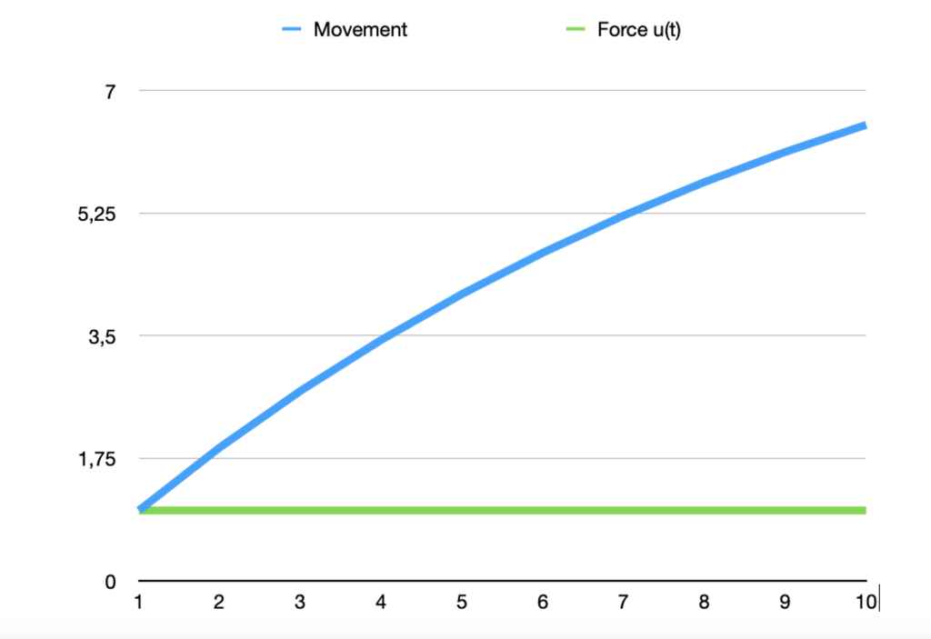
Figure 1: Ballistic movement

Figure 2 shows a computed ballistic movement from the first movement x(t0) = 0, where the inertia rate a = 0.9 and the external force u(t) = 1. The computed, x(t), has a ballistic movement, like a cannonball. The movement, x(t), will grow to infinity for a > 1, and move to zero for a < 1.

Newton dynamics was a new scientific framework. It became possible to test models of nature. Slowly this new science developed a new framework of understanding motions in nature. A new concept to understand dynamics in nature. The Newton dynamic paradigm can preserve information about all past movements. Future movements are not known. It is like driving a car, by looking in a mirror. The next turning point is unknown. This property explains why a model mat be trained to explain past variation but cannot compute future variations. To compute future variation, we need deterministic information about the final movement.

Case 2: Global warming dynamics

Case 2: Global warming dynamics

Accumulation of heat in the atmosphere may be explained by the simplified model: 

dX_gw(t)/dt = A_gw*X_gw(t) +U_agw(t) +U_ngw(t)

where X_gw(t) represents the accumulated global warming, A_gw the loss rate, U_agw(t) anthropogenic forced global warming and U_ngw(t) natural forced global warming. By this simple model, global warming may be computed, if [A_gw, X_gw(t), U_agw(t), U_ngw(t)] are known. The external sources U_agw(t) and U_ngw(t) have time variations. Then the model must be expanded to a system model.

CO₂ forced global warming

Jay D Forrester worked with servo-technical systems and was one of those who helped develop the first digital computers during the Second World War. Forrester believed management subjects at universities and companies were dominated by psychologists, political and social dogmas with little scientific grounding. He believed subjects such as administration, management and social planning had not taken part in the knowledge development in mathematical modeling from cybernetics. He was particularly interested in demonstrating the impact of dynamics in industrial and social systems.

The Forrester paradigm was based on accumulation and flow of materials and economy as dynamic systems. This was a new way of understanding dynamics in a chain of events from a first cause to a final cause. Before Forrester, system dynamic models were used in physics, electronics, and automation. Forrester expanded the concept to flow of information, materials, orders, personnel, and capital. Models, based on flow and accumulation, was expanded to models of Urban Dynamics, Industrial Dynamics, and World Dynamics.

Case 3: CO₂ forced global warming

Global warming dynamics may be explained by the simplified model:

dX_gw(t)/dt = A_gw*X_g(t) + U_agw(t) + U_ngw(t)

The Arrhenius greenhouse hypothesis is explained by the simplified model:

            U_agw(t) = K_co2(t) X_co2(t)

Global atmospheric CO₂ dynamics may be explained by the simple model:

dX_co2(t)/dt = A_co2*X_co2(t) + U_acco2(t) + U_nco2(t)

where K_co2(t) represent CO₂ impact on global warming. By this simple model, future global warming, X_gw(t), may be computed, if [A_gw, U_agw(t), U_ngw(t), X_gw(t₀), K_co2(t)], and [A_co2, U_aco2(t), U_nco2(t), X_co2(t₀)] are known. If not, unknown model parameter must be estimated. 

CO₂ forced global warming is based on the simple idea that global temperature and global CO₂ are autonomous dynamic systems, and a linear relation between CO₂ dynamics and global temperature. Global warming, X_gw(t), is reduced when anthropogenic forced CO₂ (U_aco2(t)) is reduced. The Arrhenius greenhouse hypothesis must be confirmed. The next problem is to control anthropogenic inflow to the atmosphere. This is a control problem. Control theory is made to control manmade systems. Control of nature is not the same.

Global warming control

Norbert Wiener (1894-1964) was one of the most significant mathematicians of his time. Wiener studied philosophy and was interested in Leibniz’s philosophy of nature as a holistic concept. He therefore saw clear similarities between servo technology and biological processes. Examples of this were the body’s regulation of heat, chemical balance, and the sensory apparatus. Wiener introduced a new way of thinking. The nature is a self-controlling system on many levels. In 1946, he formulated the term cybernetics from the Greek word kybernetes, which means “helmsman”. The cybernetics paradigm became a  new way of understanding nature.

Wiener’s work soon gained great importance for several new disciplines. Modeling of nerve cells formed the basis for artificial intelligence, the study of frequency spectrum in cybernetic systems became important for a new understanding of the dynamics of economic and ecological systems. Concepts based on control theory were thereby significantly further developed to not understand dynamics inn nature.

Case 4: Global warming control

Global warming control, by the Arrhenius greenhouse hypothesis, may be explained a simple cybernetic control system:

dX_gw(t)/dt = A_gw*X_gw(t) + U_aco2(t)+U_nco2(t)

            U_aco2(t) = K_co2(t) X_co2(t)

dX_co2(t)/dt = A_co2*X_co2(t) + U_aco2(t) +U_nco2(t)

            U_co2(t) = K(U_ref(t)-X_aco2(t)),

where U_ref(t) represents a desired CO₂ level, X_co2(t) represents monitored CO₂, and U_nco2(t) represents natural CO₂inflow. To control a dynamic system, the system must be controllable and observable. 

A system is controllable if it possible to move the system states in the control direction. Atmospheric CO₂ is controllable if U_aco2(t) > U_nco2(t). Anthropogenic forced CO₂ is estimated to: U_aco2(t) = 0.06 U_nco2(t). This large difference reveals that atmospheric CO₂ is not controllable. The autonomous CO₂ loss rate, A_co2, is estimated to reduces CO₂ by 50% in approximately 7 years. This fast CO₂ reduction reveals that CO₂ inflow and outflow is controlled by an unknown source. 

Disturbance from an unknown source

“Chance ” manifests itself in many forms,
Brings many matters to surprising ends;
The things we thought would happen do not happen;

The unexpected “Chance” makes possible:
And that is what is happening all the time” 

–Euripides, 5th century BC, at the end of Medea. 

Case 5: Disturbance from an unknown source

Global warming and CO2 have model and monitored disturbance from unknown sources. The simple model must be updated.

dY_gw(t)/dt = A_g*Y_gw(t) +U_agw(t)+U_ngw(t))+E_gwe(t)

Y_gw(t) = X_gw(t) + W_gw(t)

U_agw(t) = K_co2(t)(Y_co2(t) +W_co2(t)), 

dY_co2(t)/dt = A_co2*Y_co2(t) + U_aco2(t) +U_nco2(t)) + E_co2(t)

Y_co2(t) = X_co2(t) + W_co2(t)

U_aco2(t) = K(U_ref(t)-Y_co2(t))

Global warming has a disturbance from an unknown source E_gwe(t). CO₂ variations has a disturbance form an unknown source E_co2(t). The unknown sourced influences the ability to control CO₂ and global warming. A system is observable if it possible to observe or estimate the current states in a dynamic system. If all major CO₂ sauces are not observable, the sources must be estimated. The current state of global warming, X_gw(t), and CO₂ X_co2(t), are position dependent on Earth.

Global warming and global CO₂ have different states on the Earth. A global representation must be represented by an estimated temperature model, W_gw(t) and a global CO₂ model W_co2(t). This mean that global warming and CO2 are not observable. A possible solution is to introduce a global grid of climate model. A set of climate models introduces a set of regional climate estimates.

The best estimate

Norbert Wiener had several friends who were some of the leading biologists of the time. They would later form the basis for what we today call artificial intelligence. During World War II, Wiener worked at MIT. He studied an artillery guidance system that follows an aircraft via a radar. His work was not adopted, but the methodological basis later gained great importance for the development of servo technology. Identifying a signal from noise in the radar formed the basis for the Wiener filter. This filter had the property that it could optimally identify a signal that was affected by disturbance from an unknown source.

Rudolf Emil Kalman (1930-) was born in Budapest, Hungary. Kalman was one of many who fled to the United States. He had a background in electronics and was particularly interested in mathematical system theory. Kalman was sitting on a train thinking about the Wiener-filter. Suddenly he came up with the idea of transferring the Wiener-filter from a frequency spectrum form to linear algebra. The result was the Kalman-filter for optimum estimate of disturbance from an unknown source. 

The Kalman-filter was a milestone in the development of modern estimation theory and represents a paradigm shift from frequency plane analysis to an analysis in the time plane. Eventually, the Kalman-filter was adopted by the Apollo program, the aerospace industry, and the process industry.

Case 6: Estimating global warming

Real values of global warming dynamics may be estimated by the simplified model:

dX_gw(t)/dt = A_gw(t)*X_gw(t) + U_agw(t) +U_ngw(t) + E_gw(t)

            Y_gw(t) = X_gw(t) + W_gw(t)

where E_gw(t) represents a global warming form an unknown source and W_gw(t) is monitored error from an unknown source. If the unknown source E_gw(t) is uncorrelated variations (white noice spectrum), the unknown source has a mean value E[W_g(t)] = W₀. This mean value may be estimated using a Kalman-filter. If the unknown source, E_gw(t), has a red spectrum (amplitude is falling by 1/frequency), the disturbance has no stationary mean value. The disturbance may have periods from minutes to thousands of years. Global warming then must be controlled by future events. If future events are unknown, global warming is not controllable. 

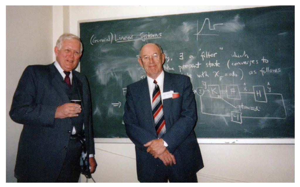
Figure 2. Jens G Balchen and Rudolf Kalman. NTNU Trondheim, September, 2009.

Thousands of scientific papers are based on  the algorithm, which has created thousands of industrial applications. Jens G Balchen created an institute at NTNU-Trondheim, based on the Kalman-filter algorithm. Kalman had a presentation of the Kalman-filter at NTNU in September 2009. In this presentation Kalman revealed that the Kalman-filter has a limitation.

The Kalman-filter has best performance if disturbances for an unknown source, W(t) , has non-correlated “white noise”. If the disturbance has a red spectrum (1/frequency), long periods will influence the estimated values. Now Kalman was studying the work from the Norwegian Ragnar Frisch. Frisch had studied statistic models of uncertainty. Kalman was looking for better models of red spectrum. To understand disturbance for an unknown source, we must identify the disturbance signature S(T, F), where T represents the cycle period spectrum, and F represents the cycle period phase relations.

Solar-lunar forced disturbance signature

A signature analysis of global temperatures has revealed that global land temperature has a solar forced signature S_so(T_so, F_so), where T_so, has periods up to 4450 years, controlled by the Jovian planets. Global sea temperature (SST) and global temperature has a sola forced signature S_so(T_so, F_so + T_so/4) and a lunar forced signature S_ln(T_ln, F_ln), where T_ln, has periods up tu 445 years. The unknown source has signatures from the solar system (Yndestad 2022a).

A signature analysis of atmospheric CO₂ from 1820 to 2020 has revealed a lunar forced signature. The signature has a coincidence to global sea surface temperature with a phase-lag of pi/2 (rad). The pi/2 (rad) phase-lag reveals a temperature forced control of CO₂ outflow into the atmosphere (Yndestad 2022b). A lunar forced signature in CO₂ variations reveals that CO₂ is not controllable.

Case 7: Solar-lunar forced global warming

Global warming has major influence from external sources which have a spectrum of solar-lunar periods. Global land temperature variations may be explained by the signature model:

            S_gw(T_gw, F_gw) = S_so(T_so, F_so),

Global sea surface temperature variation may be explained by the signature:

            S_sst(T_sst, F_sst) = S_so(T_so, F_so+T_so/4) + S_so(T_so, F_so),

Atmospheric CO2 variations mat be explained by the signature:

            S_co2(T_co2, F_co2) = S_sst(T_sst, F_sst+T_sst/4),

So why has climate science not succeeded to develop reliable climate models? The simple answer is that climate is controlled by solar-lunar periods. 

Literature

1. Parisavtalen: https://snl.no/Parisavtalen
2. Norbert Wiener: https://en.wikipedia.org/wiki/Norbert_Wiener
3. Rudolf E Kalman: https://en.wikipedia.org/wiki/Rudolf_E._Kálmán
4. Kalman-filter https://en.wikipedia.org/wiki/Kalman_filter
5. Beck, Ernst-Georg, 2022: Reconstruction of Atmospheric CO2 Background Levels since 1826 from Direct Measurements near Ground. Science of Climate Change, 2, 148-211. https://doi.org/10.53234/scc202112/16
6. Anderson Thomas R., Hawkins Ed, Jones Philip D., 2016: CO2, the greenhouse effect and global warming: from the pioneering work of Arrhenius and Callendar to today’s Earth System Models, Endeavour, V olume 40, Issue 3, 2016, Pages 178-187, ISSN 0160-9327, https://doi.org/10.1016/j.endeavour.2016.07.002.
7. Yndestad Harald, 2022a: Jovian Planets and Lunar Nodal Cycles in the Earth’s Climate. Variability, Frontiers in Astronomy and Space Sciences, 10 May. https://www.frontiersin.org/article/10.3389/fspas.2022.839794.
8. Yndestad Harald, 2022b: Lunar Forced Mauna Loa and Atlantic CO2 Variability. Science of Climate Change, Vol. 2.3 (2022) pp. 258-274. https://doi.org/10.53234/scc202212/13
9. Lunar forced climate: https://www.climateclock.no/2021/03/lunar-forced-global-climate/
10. Solen varierer over 4450 år: https://www.climateclock.no/2022/10/tsi-variasjoner/