
Climate variations leaves its footprints in nature. What we see from recorded events are apparently random climate changes over time. Records of past events hide its information about the source of climate change, and what to expect for the future. The cause of past climate has to be decoded from climate footprints. To understand the footprints of climate change, we must understand the nature´s language. The nature´s language is mathematics.
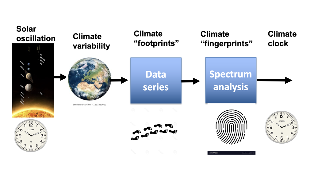
Figure 1 Steps in climate signature identification
Figure 1 shows an example of how we can reveal the source of changes in nature. Periodic cycles in the solar system cause periodic changes in radiation from the sun. Periodic changes in radiation from the sun leave their mark on nature. Traces from previous climate changes are registered as climate change’s “footprint”. The measurements’ “footprint” then represents the characteristics of past climate changes. The footprint signature reveals the footprint source. If the source has stationary cycles from the solar system, the climate periods behave like a clock. A Climate Clock.
The Tide Predictor Machine
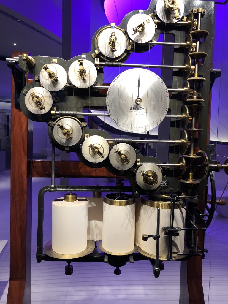
Figure 2 The Tide Predictor Machin
Lord Kelvin (1824-1907) began studying tide tables for ships sailing on the Thames to London. Using Fourier’s method, he found that the tide tables had periodic changes, consistent with periodic changes in the solar system. Periods in the solar system, which were well known. He could then calculate future changes in the tide,
Based on this discovery, in 1872 he developed a mechanical computer that calculated the tides over a period of one year. This Tide Predictor Machine was in use right up until the 1960s. Lord Kelvin had discovered that if the signature of a data series has a deterministic source, we can predict future events, to control future events.
Fourier spectrum signature
Baron Jean-Baptiste-Joseph Fourier (1768-1830) was a French mathematician best known for developing a mathematical analysis of heat propagation. Fourier took part in Napoleon’s campaign to Egypt in 1798. When Napoleon traveled on to Palestine and fought against the Assyrians, Fourier stayed back in Cairo where he studied mathematics for three years. Fourier was concerned with the properties of heat.
One day he saw a blacksmith making an anchor ring. When the anchor ring was placed in the sand to cool, he noticed the heat was not equally distributed around the anker ring. There were dark, red, and white heat waves over the ring. At one place there was a sharp separation between the hottest and coldest area on the ring. He concluded that heat distribution was controlled by a sum of sinusoidal cycle thermal waves. Temperature variations was distributed by interference between standing thermals waves.
In 1807 Fourier formulated his theory and in 1822 he published the book “The analytical theory of heat”. In the past 100 years, the Fourier transform became a new scientific approach to study cycle movements in nature. The Fourier transform created the scientific basis for new subjects such as electronics, telecommunications, acoustics, seismic, optics, artificial intelligence, etc.
The Fourier-transform
Fourier discovered that a series of n numbers, x(t) = [x(t0)…x(tn)], can be represented by a frequency spectrum: X(j2p/T) = [a1sin(2π(t- t1)/T1)… aN/2sin(2π(t-tN/2)/TN/2)], where ai represents the amplitude of a sine period sin(2π(t-ti)/Ti), with period time Ti and phase ti. This means that all data series can be classified with a signature S(A, T) with a frequency spectrum, which have the dominant periods: T = [T1…Tn/2] and amplitude variations A = [a1…an/2]. The Fourier transform is based on a cross-correlation between the data series x(t) and a set of sine periods sin(2π(t- i1)/Ti).
Example 1. Cycle periods in noisy time series
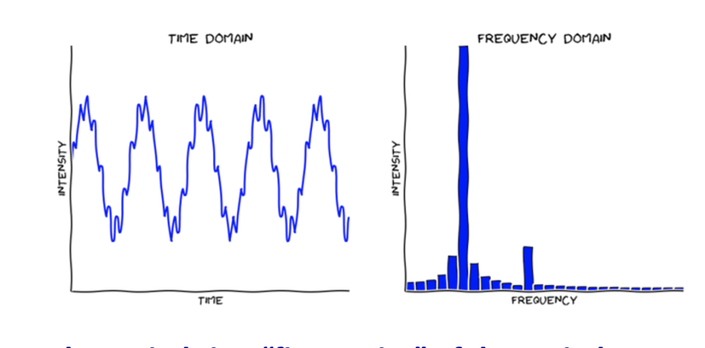
Figure 3 Time series and Fourier transformed time series
Figure 3 shows the computed time-series: x(t) = sin(2pi*t /T) + v(t); where v(t) is random non-correlated “noise”. The Fourier transformed spectrum has identified the frequency period f = 1/T and the distributed “white” spectrum.
Fourier signature limitations
The Fourier paradigm was a new scientific approach to understand movements in nature. After Fourier science moved in two different directions. Prediction by models is based on a Newton approach, and predictions by data based on a Fourier approach.
The idea was not fully understood by the great mathematicians of the time. During the last fifty years, the Fourier paradigm has been widely used in hundreds of scientific papers. In climate science the Fourier paradigm has been uses in a number paper to identify stationary periods in long time series.
The Fourier transform represents a basic method for identifying the signature in time series. At the same time, one must be aware that all methods have their limitations, which limit the method’s ability to identify the signature. The Fourier spectrum paradigm has some limitations. The most important limitations are:
- The sampling theorem: A time-series of N elements, can identify only N/2 periods.
- Lost phase information: Single everts has lost the phase-information (the position).
- Sidelobes: Beginning and the end of a time-series introduces false periods.
- Physic representation: Sinus periods may not represent correlation to physics in nature.
- Period interference: False periods for interference between two or more periods.
- Temporary stationary periods: Estimated periods may be based on temporary stationary periods.
The most serious problem is the loss of phase information. The timing of periodic changes in time series.
Example 2. The 60-year cycle
A 60-cycle has been identified in climate time series. It has been suggested that the source is the planet Saturn. Saturn has a period Tsa = 29.45 years and a sub-harmonic period of 2Tsa = 58.9 years. A coincidence between climate periods and planet periods does not prove that Saturn is the source of the 60-year climate period. Period coincidences does not prove a source. The Jovian planets, Jupiter, Saturn, Uranus, and Neptune have hundreds of period combinations. The second source of error is the Fourier transform. Global temperature has 150 temperature samples from 1850 to 2000. The Fourier transform estimates periods up to 150/2 = 75 years. The 75-period is based on only 2 samples.
A possible source of the estimated 60-year cycle is the Lunar nodal cycle Tln = 18.6 years. The Lunar cycle has sub-harmonic periods of 3Tln=55 years, and 4Tln = 74 years. The Fourier transform cannot separate a 55-year period from a 74-year period, in a 150-year time series. To identify the source of a climate cycle, we need the period phase information.
This means that Fourier transformed is an outdated method for a complete climate signature identification. In the 1990s, the oil industry developed a new method called wavelet spectrum analysis. This method has been crucial to identify stationary climate periods in the Climate Clock framework.